Vectors & Parametric Equations
Your phone’s GPS uses linear combinations constantly! When calculating your position, it takes signals from multiple satellites and combines them with different weights to pinpoint your location.
In animation and gaming, characters move smoothly because their positions are calculated as weighted combinations of keyframe positions — exactly what we’re learning today!
This concept (linear combinations) is also the foundation of machine learning and AI. Neural networks are essentially very complicated linear combinations!
Topics Covered
- Trisecting points on a line segment
- Weighted averages as linear combinations
- Vector notation: \(\vec{AP} = \lambda \cdot \vec{AB}\)
- Parametric equations of a line
- Extension to 3D
A regular average treats everything equally: \[\text{Average of 3 and 9} = \frac{3 + 9}{2} = 6\]
A weighted average gives more importance to one side:
- “75% of the way from 3 to 9” = \(0.25 \times 3 + 0.75 \times 9 = 7.5\)
- “33% of the way from 3 to 9” = \(0.67 \times 3 + 0.33 \times 9 = 5.0\)
The weights always add up to 1 (100%). This works for coordinates too!
Lecture Video
Key Video Frames
Points as Linear Combinations
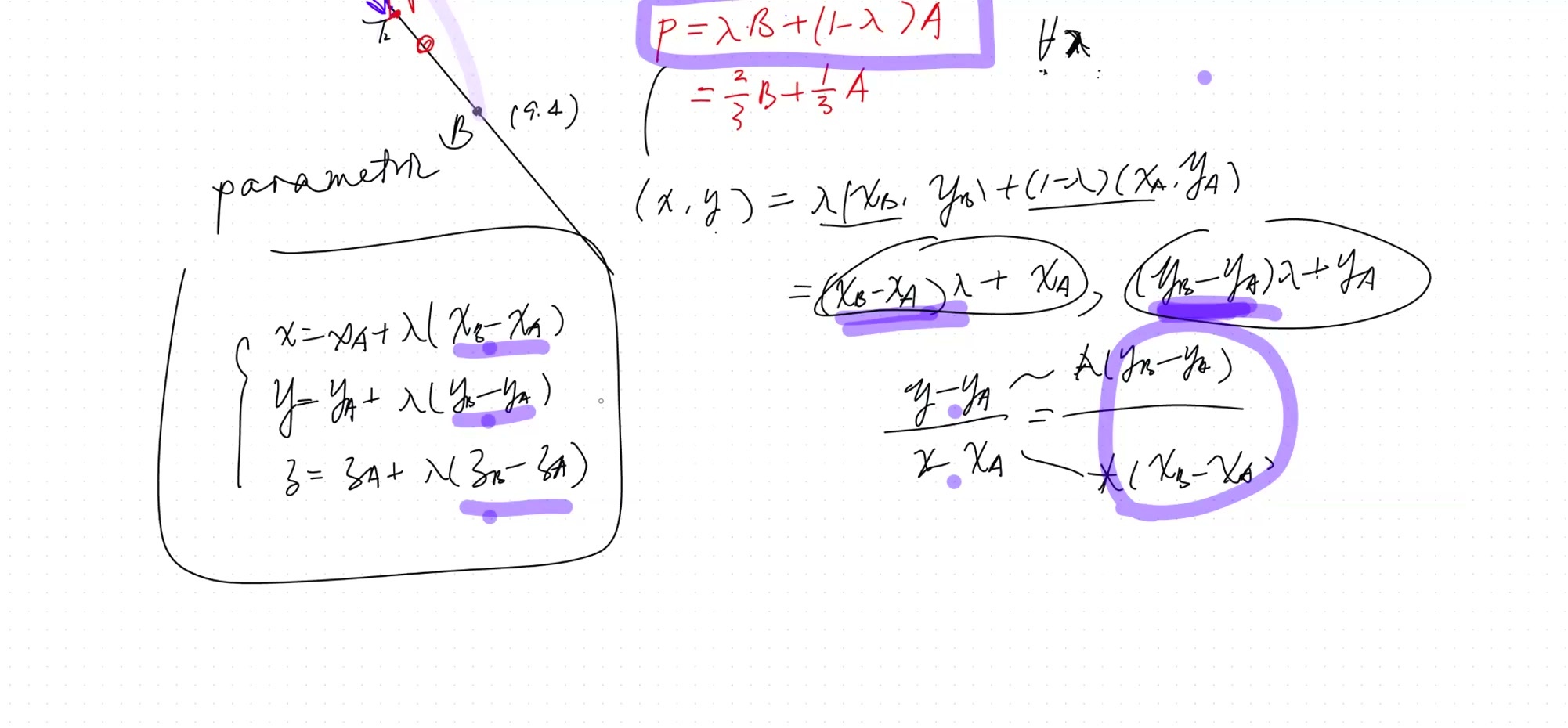
Given endpoints \(A\) and \(B\), any point \(P\) on line \(AB\) can be written:
\[P = \lambda B + (1 - \lambda) A\]
Think of \(\lambda\) as a progress bar from \(A\) to \(B\).
- \(\lambda = 0\): at point \(A\)
- \(\lambda = 1\): at point \(B\)
- \(0 < \lambda < 1\): between \(A\) and \(B\)
- \(\lambda < 0\) or \(\lambda > 1\): outside segment \(AB\)
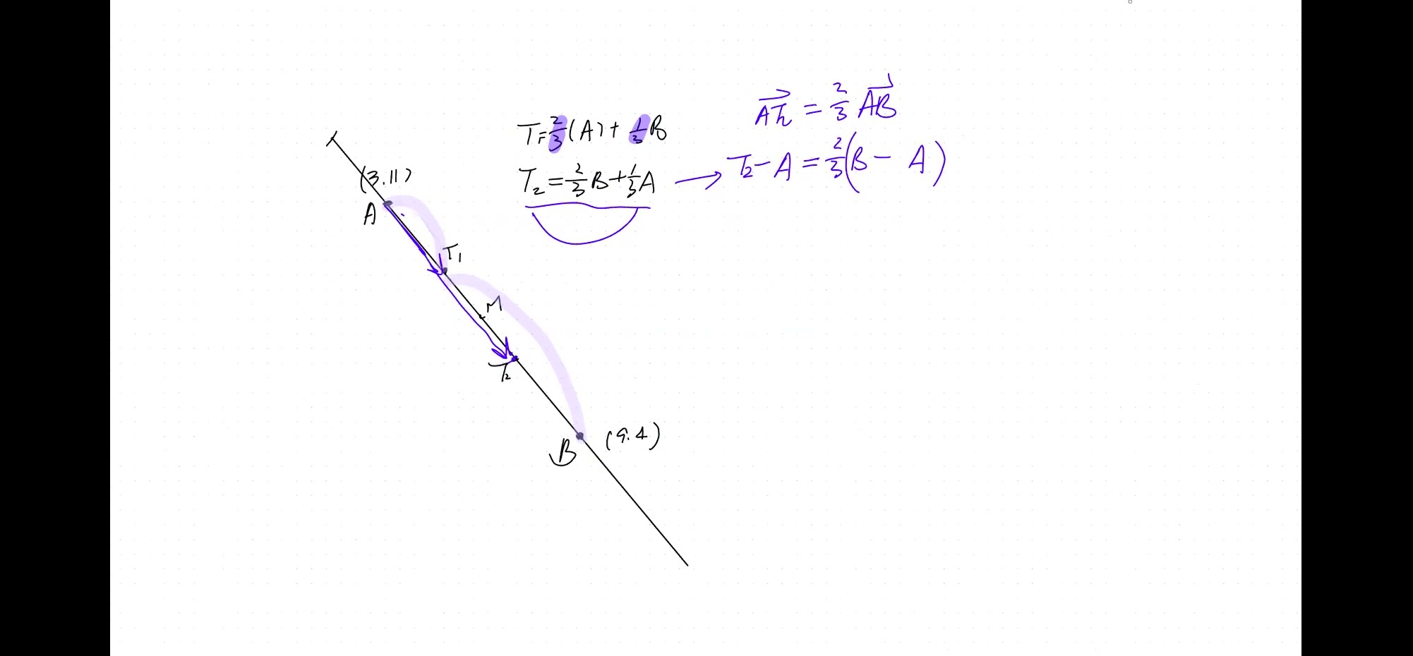
Example 1: Find trisecting points
Given: \(A = (3, 11)\), \(B = (9, 4)\)
Trisector \(T_1\) (closer to \(A\), \(\lambda = 1/3\)): \[T_1 = \frac{2}{3}A + \frac{1}{3}B = (5, \tfrac{26}{3})\]
Trisector \(T_2\) (closer to \(B\), \(\lambda = 2/3\)): \[T_2 = \frac{1}{3}A + \frac{2}{3}B = (7, \tfrac{19}{3})\]
Rule: Closer to a point → give more weight to that point
Drag \(\lambda\) to move the point along the line:
Instead of writing \(y\) in terms of \(x\) (like \(y = 2x + 1\)), we write both \(x\) and \(y\) in terms of a third variable \(\lambda\) (the “parameter”):
\[x = x_A + \lambda(x_B - x_A), \quad y = y_A + \lambda(y_B - y_A)\]
Think of \(\lambda\) as time. As time goes from 0 to 1, the point travels from \(A\) to \(B\).
Why is this useful? It works in ANY number of dimensions! The slope formula only works in 2D, but parametric equations work in 2D, 3D, 4D, or any dimension.
Parametric Equations
The parametric form of a line through \(A(x_A, y_A)\) and \(B(x_B, y_B)\):
\[\begin{cases} x = x_A + \lambda(x_B - x_A) \\ y = y_A + \lambda(y_B - y_A) \end{cases}\]
Eliminating \(\lambda\) recovers the familiar slope-intercept form:
\[\frac{y - y_A}{x - x_A} = \frac{y_B - y_A}{x_B - x_A} = m \text{ (slope)}\]
Extension to 3D
Just add a \(z\) equation — no slope needed!
\[\begin{cases} x = x_A + \lambda(x_B - x_A) \\ y = y_A + \lambda(y_B - y_A) \\ z = z_A + \lambda(z_B - z_A) \end{cases}\]
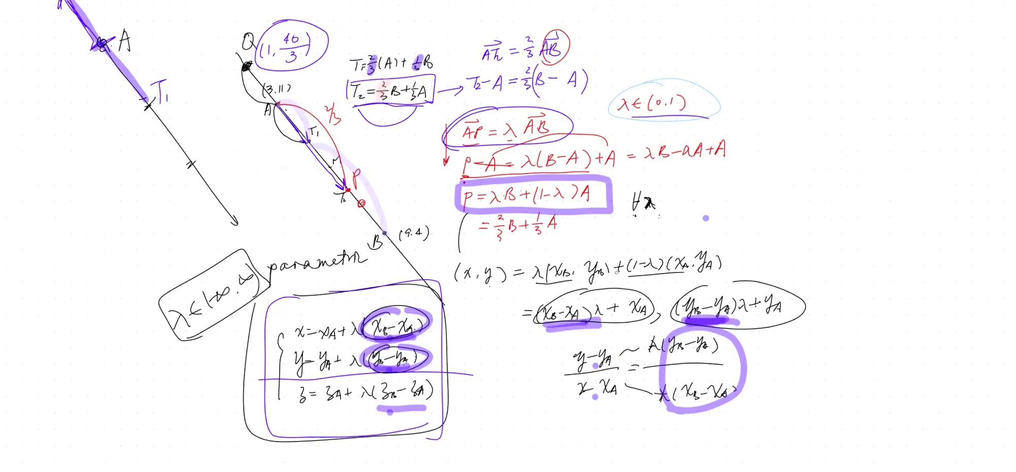
External points
Given: \(A = (3, 11)\), \(B = (9, 4)\), point \(Q\) outside \(AB\) on side of \(A\), with \(|AQ| = \frac{1}{3}|AB|\)
\[\vec{AQ} = -\frac{1}{3}\vec{AB}\] (Negative because \(Q\) is on the opposite side from \(B\))
\[Q = A - \frac{1}{3}(B - A) = (1, \tfrac{40}{3})\]
Cheat Sheet
| Concept | Formula |
|---|---|
| Point as weighted average | \(P = (1-\lambda)A + \lambda B\) |
| Midpoint (\(\lambda = 1/2\)) | \(M = \frac{1}{2}(A + B)\) |
| Trisector near \(A\) (\(\lambda = 1/3\)) | \(T = \frac{2}{3}A + \frac{1}{3}B\) |
| Interior point | \(0 < \lambda < 1\) |
| Exterior point | \(\lambda < 0\) or \(\lambda > 1\) |
Remember: The weight closer to a point means you’re giving MORE weight to that point. It’s like a tug-of-war: the stronger pull wins!